Introduction
Quantum Computer has many advantages over classical computers. Moreover, one crucial problem many applications face is searching for a large dataset. This problem becomes substantial when we have an unstructured dataset. Grover’s algorithm shows the quadratic speed-up performance on unstructured search problems.
Unstructured Search
Suppose we have an extensive list of N items. And, we need to find one item on the list. We will call this item the Winner w. In classical computing, we need to match the item in the list one by one to find the winner element. On an average case, we can do this in N/2 times, and for the worst-case N times. However, On the quantum computer, we can find the item in roughly √N steps with Grover’s algorithm. The quadratic speed is a substantial time-saver for searching for an element in the long list. The imperative function of Grover’s Algorithm is the Amplitude Amplification.
The Algorithm
To understand Grover’s Algorithm we need to first understand what is amplitude amplification. Amplitude Amplification By using the amplitude amplification function, the quantum computer mainly enhances the Winner’s amplitude; on the other hand, it reduces the amplitude of other items. So that in the final state, it will return the correct item with high certainty. Amplitude amplification will have two parts.
1. Oracle reflection
2. Diffuser operation
1. Oracle Reflection:
First, we apply the oracle reflection Uf to the state |s>.

Geometrically this corresponds to a reflection of the state |s⟩ about |s′⟩. This transformation means that the amplitude in front of the |w⟩ state becomes negative, which in turn means that the average amplitude (indicated by a dashed line) has been lowered.
2. Diffuser Operation
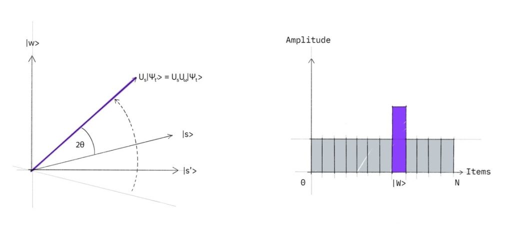
Once we have our inverted phase, we’re going to invert all amplitudes around the mean. This transformation rotates the initial state |s> closer to the winner |w>
The action of the reflection in the amplitude bar diagram can be understood as a reflection of the average amplitude. Since the average amplitude has been lowered by the first reflection, this transformation boosts the negative amplitude of |w⟩ to roughly three times its original value, while it decreases the other amplitudes. This procedure will be repeated several times.
Now the question comes how many times do we need to apply the rotation? It turns out that roughly √N rotations suffice. This becomes clear when looking at the amplitudes of the state |ψ⟩. We can see that the amplitude of |w⟩ grows linearly with the number of applications. However, since we are dealing with amplitudes and not probabilities, the vector space’s dimension enters as a square root. Therefore it is the amplitude and not just the probability, that is being amplified in this procedure.
To summarize Grover’s Algorithm will have the following steps:
Step 1: Initialization
Step 2: Grover’s Amplitude Amplification (repeat √N times)
Step 2.1: Oracle
Step 2.2: Diffuser
Step 3: Measurement
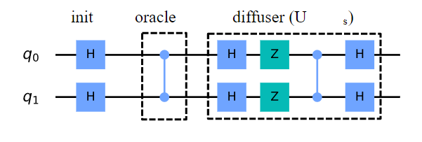
INITIALIZATION
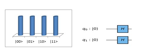
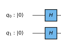
The first part of the algorithm commonly referred to as the initialization basically put the quantum computer into an equal superposition of all the possible states.
Implementation on Qsim: 2 Qubits
First, we will implement the case where N=4 is realized with 2 qubits. Let us say my winner state is |11> [3]. In this particular case, only one rotation is required to rotate the initial state |s⟩ to the winner |w⟩:
Step1: Initialization
Hadamard gate is used for states to be in an equal superposition.
Step 2:
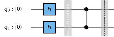
Step 2.1: Oracle
For this example, our oracle is simply the controlled-Z gate:
Step 2.2: Diffuser
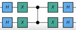
Complete Circuit for |w⟩=|11⟩
For this particular case where N=4 only one rotation is required, we can combine the above components to build the full circuit for Grover’s algorithm for the case |w⟩=|11⟩:
Let’s implement Grover’s Algorithm on QSim for the above case of 2 qubits where |w⟩=|11⟩
# Grover's Algorithm with two- qubit
from qiskit import QuantumRegister, ClassicalRegister
from qiskit import QuantumCircuit, execute, BasicAer
import numpy as np


#Options & Noise goes here - Don't change options variable name & block
options = {
'plot': True,
"rotation_error": {'rx':[1.0, 0.0], 'ry':[1.0, 0.0], 'rz':[1.0,0.0]},
"tsp_model_error": [1.0, 0.0],
"thermal_factor": 1.0,
"decoherence_factor": 1.0,
"depolarization_factor": 1.0,
"bell_depolarization_factor": 1.0,
"decay_factor": 1.0,
}
#####   Write your code after this line  ######

### Create a quantum Circuit with two qubits ###
q = QuantumRegister(2)
c = ClassicalRegister(2)
circuit = QuantumCircuit(q,c)

### Step 1: Initialization  ###
circuit.h([0,1])
circuit.barrier()

### Step 2: Oracle W=11 ###
circuit.cz(0,1)
circuit.barrier()

### Step 3: Grover’s Diffusion Operator  ###
circuit.h([0,1])
circuit.x([0,1])
circuit.cz(0,1)
circuit.x([0,1])
circuit.h([0,1])


### Step 4: Measurement  ###
circuit.measure(q,c,basis="Ensemble",add_param="Z")
backend = BasicAer.get_backend('dm_simulator')

### Execute the circuit  ###
job = execute(circuit, backend=backend, **options)
job_result = job.result()

prob = print(job_result.results[0].data.ensemble_probability)
With the above code, we will be able to generate the following circuit

After submitting the job we can get the following output
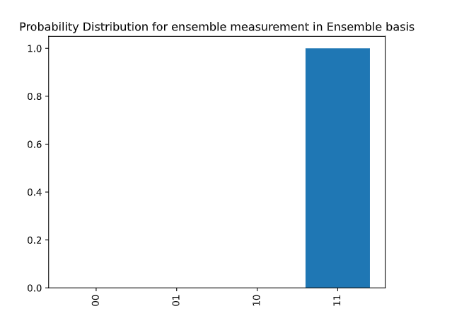
As we can see in the output, the amplitude of every state that is not |11⟩ is 0, this means we have a 100% chance of measuring |11⟩ . This is the case when there was not error in the system. we can introduce some error in the system and try to run the job.
Implementation on Qsim: 3 Qubits
Now, we will implement Grover’s Algorithm with 3 qubits where |w⟩=|111⟩
### Grover's Algorithm with three- qubit ###
from qiskit import QuantumRegister, ClassicalRegister
from qiskit import QuantumCircuit, execute, BasicAer
import numpy as np


#Options & Noise goes here - Don't change options variable name & block
options = {
'plot': True,
"rotation_error": {'rx':[1.0, 0.0], 'ry':[1.0, 0.0], 'rz':[1.0,0.0]},
"tsp_model_error": [1.0, 0.0],
"thermal_factor": 1.0,
"decoherence_factor": 1.0,
"depolarization_factor": 1.0,
"bell_depolarization_factor": 1.0,
"decay_factor": 1.0,
}
#####   Write your code after this line  ######

### Create a quantum Circuit with three qubits ###
q = QuantumRegister(3)
c = ClassicalRegister(3)
circuit = QuantumCircuit(q,c)


### Step 1: Initialization  ###
circuit.h([0,1,2])
circuit.barrier()

### Step 2: Oracle  HXH = X###
circuit.h(2)
circuit.ccx(0,1,2)
circuit.h(2)
circuit.barrier()
### Step 3: Grover’s Diffusion Operator  ###
circuit.h([0,1,2])
circuit.x([0,1,2])
circuit.h(2)
circuit.ccx(0,1,2)
circuit.h(2)
circuit.x([0,1,2])
circuit.h([0,1,2])
circuit.barrier()
### Second Iteration ###
### Step 2: Oracle  HXH = X###
circuit.h(2)
circuit.ccx(0,1,2)
circuit.h(2)
circuit.barrier()
### Step 3: Grover’s Diffusion Operator  ###
circuit.h([0,1,2])
circuit.x([0,1,2])
circuit.h(2)
circuit.ccx(0,1,2)
circuit.h(2)
circuit.x([0,1,2])
circuit.h([0,1,2])
circuit.barrier()
### Step 4: Measurement  ###
circuit.measure(q,c,basis="Ensemble",add_param="Z")
backend = BasicAer.get_backend('dm_simulator')

### Execute the circuit  ###
job = execute(circuit, backend=backend, **options)
job_result = job.result()
prob = print(job_result.results[0].data.ensemble_probability)
#The above code will create the following circuit
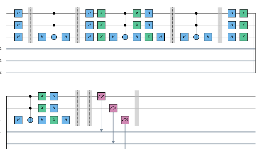
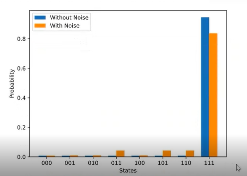
Once we’ll submit the job it will give us the following output. As we run the amplitude amplification two times, we can see that amplitude of every state that is not |111⟩ is reduced, this means we have a maximum chance of measuring |111⟩

Implement circuit with Error in the system
Let us try to run the same code with errors in the system. We will get the following output. we can see due to error amplitude of the winning state is reduced.
References:
1. L. K. Grover (1996), “A fast quantum mechanical algorithm for database search”, Proceedings of the 28th Annual ACM Symposium on the Theory of Computing (STOC 1996), doi:10.1145/237814.237866, arXiv:quant-ph/9605043
2. C. Figgatt, D. Maslov, K. A. Landsman, N. M. Linke, S. Debnath & C. Monroe (2017), “Complete 3-Qubit Grover search on a programmable quantum computer”, Nature Communications, Vol 8, Art 1918, doi:10.1038/s41467-017-01904-7, arXiv:1703.10535
3. Qiskit textbook https://qiskit.org/textbook/preface.html